Modeling Data Durability and Availability
Outline
Acknowledgements:
Ian Davies, Mike Barrell, John Bent, and Iman Anvari

- Press F11 for full screen
- Ctrl +/- to fit the content into the browser
- Use arrow keys to navigate the slides
- Table of contents button on the left bottom
- Printable PDF:
- Recorded session:
-
Fragments: Enable or disable fragment transitions within slides
-
Modeling Failures
- Weibull Distribution
-
Erasure Coding(EC)
-
General formalism,
RAID Redundant Array of Inexpensive Disks5& 6
-
General formalism,
-
Hard Errors (
UREs UnRecoverable Errors)
- Modeling durability with UREs
-
Distributed Parity
-
Improving data durability with
ADAPT Autonomic Distributed Allocation Protection Technology
- Multi-Layer EC
- Improving durability with two layers of EC
- Availability
- Modeling data availability
- Appendix
-
MACH2 Exos® 2X14, Seagate’s Dual actuator driveandReMan ReManufacturing drives with head failures
Goals & Summary
Goals- Provide a quick review of available models to compute data durability,
- Present an accurate and rigorous model,
- Establish a common language to compute these metrics.
SummaryThe durability of data in storage systems is determined by physical device failure rates. A typical storage system has multiple storage devices, which significantly increases the likelihood of failures. In order to improve the reliability, data redundancy is added to the system so that it becomes possible to recover data on a failed storage device from the parities stored on the remaining healthy devices. For example, in the case of Redundant Array of Inexpensive Disks (RAID), adding one redundancy ensures data robustness to one failure, whereas adding two redundancies will provide robustness against two simultaneous failures[3]. The data durability can be further increased by implementing sophisticated erasure coding schemes[4]–[8] and also by prioritizing the recovery of critically damaged data stripes[9]. In all of these schemes, the durability critically depends on how fast the data on a failed device can be reconstructed to restore the redundancy.
-
The durability and availability of data can be predicted accurately with Markov Chains:
- Based on rigorous math, and verified with Monte Carlo simulations.
- Supports Distributed Parity, ReMan, UREs, Weibull failure modes, and multi-layer EC.
- Developed in collaboration with the CORTX architects & sales team.
-
Advanced features, such as Online ReMan, can be modeled too:
- We continue to work on modeling latest and greatest CORTX features.
Visualizing failure distributions
In the interactive plot below, \(\alpha\) and \(\beta\) values can be adjusted. The toggles on the right change the scales.![An interactive plot of Weibull distributions defined in Eqs.<span class='myeqref'> \@ref(eq:weipdf) </span>,<span class='myeqref'> \@ref(eq:weicdf) </span> and <span class='myeqref'>\@ref(eq:weihazard)</span>. Use the toggles for linear/log scales. <span class='plus'>... [+]</span> <span class='expanded-caption'> The vertical dashed lines mark the value $t=\alpha$, and the horizontal one on $F$ marks the value $0.63$. The $y$ axis can be transformed to $ln\left[-ln(1-F_{\alpha,\beta})\right]$, and the time axis can be transformed to $ln(t)$. The effect of $\beta$ on $F$ is best observed with the log time scale, and $y$ in the probability scale: notice how $F_{\alpha,\beta}$ becomes a line with the slope $\beta$. Selecting the log scale for time and linear scale for the $y$ axis, shows that the changing scale parameter $\alpha$ moves the functions horizontally while preserving their shapes.</span>](placeholder.png)
An interactive plot of Weibull distributions defined in Eqs. @ref(eq:weipdf) , @ref(eq:weicdf) and @ref(eq:weihazard). Use the toggles for linear/log scales. … [+]
A drive will contain \(N\) heads and other components. We will model the drive as a device with two competing failure modes, one of which is ReMan’able while the other is not.
- It is important to understand how the storage devices fail. Weibull is typically a good fit.
- No matter how reliable individual devices are, failures are inevitable.
Erasure Coding
![A brief timeline of the erasure coding. <span class='plus'>... [+]</span> <span class='expanded-caption'> Replication has very poor capacity efficieny. RAID5(6) provides protection against one(two) failure(s). Seagate enclosures can be used to declustered parity as well as erasure coding across network. Durability and availablity can be further improved by implementing Multi-layer erasure coding. Most of the method shown in this figure will be discussed in detail in this presentation. </span> Credit:John Bent](cortx.png)
A brief timeline of the erasure coding. … [+] Credit:John Bent
- The simplest way of creating redundancy is replication, but this has a very poor capacity efficiency.
- RAID 5 and Raid 6 introduce parities to protect data against device failures.
- Seagate enclosures supports declustered RAID6, which can be coupled with a top layer EC in CORTX to get the highest durability with best capacity efficiency.
RAID 5 & 6 (with URE)
A Symbolic representation of the RAID including URE failures. Use the input sliders to change the number of drives or the redundancy. … [+]
-
The red arrows represent drive failures. Rate is scaled with the total number of drives:
- \(\lambda\) is the failure rate per drive, and \(n\lambda\) is the total failure rate for \(n\) drives.
- The arrow denoted with \(h\) represents the data loss due to UREs- to be discussed in more detail later.
-
The green arrows represent repairs. Failed drives are replaced, and data is rebuilt.
- The repair time, \(1/\mu\), depends on capacity and DR. It may be as long as several days.
-
Data is lost when the system moves to the right-most state.
- Key metric: Mean Time to Data Loss (MTTDL): it is a function of \(n\), \(c\), \(\lambda\), \(\mu\), drive capacity and \({\rm UER}\).
The BackBlaze Model
This is a model introduced by [11], [12].
(\(n\)) drives , capacity(\(C\)):TB, redundancy(\(c\)):, recovery speed (\(S\)): MB/s, and AFR:%.
[11], [12].
(\(n\)) drives , capacity(\(C\)):TB, redundancy(\(c\)):, recovery speed (\(S\)): MB/s, and AFR:%.- The recovery time from a drive failure is: \(T\equiv\frac{C}{S}\)= days.
-
The AFR value can be converted to the failure rate as: \(\lambda=-\frac{\rm{ln}(1-\rm{AFR})}{\rm{ year}}\simeq\frac{\rm{AFR}}{\,\rm{ year}}\)= .
- The probability of a given drive to fail in days is: \(p_f\equiv\lambda T\)= .
- The system will not lose data when there are at most failures in days.
- The probability of not losing data in days is: \(p_\rm{no-loss}=\sum_{i=0}^c \binom{n}{i} (p_f)^i(1-p_f)^{n-i}\) =
- There are \(N_F=\frac{365}{T}\)= such frames in a year.
- The probability of not losing data in a year is: \((p_\rm{no-loss})^{N_F}\) =
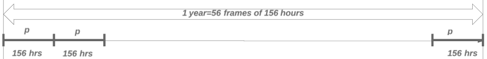
An illustration of the time frames.
- This model is still simple, but… it has a few issues:
- The segmentation of a year into chunks of days implies that data is lost only when failures happen in a given frame. The cases of failures within in days but spanning two subsequent frames are missed.
- It is implicitly assumed that every frame starts with a -redundant system. In reality, there may be up to ongoing repairs exiting the previous frame, and a single drive failure early in the next frame will cause data loss.
- Ignoring UREs, BackBlaze model works reasonably well in the low AFR limit (up to a factor of \(\sim2\)).
- Including UREs will reduce the data durability by nines.
The most intuitive model
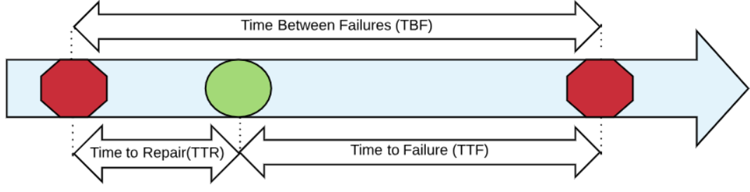
An illustration of the time scales.
- Figure plotref_avaldef_NTT shows the time scales in a repairable system.
- A system of \(n\) drives has the Mean Time To Failure: \(\rm{MTTF}=1/(n \lambda).\)
- A failed drive is replaced, and rebuilt. Mean Time To Repair: \(\rm{MTTR}=1/\mu.\)
- Fraction of the time spent for repair: \(\frac{{\rm MTTR}}{{\rm MTTF}+{\rm MTTR} }\)
- Fraction of the time spent for repair: \(\frac{{\rm MTTR}}{{\rm MTTF}+{\rm MTTR} }\simeq \frac{{\rm MTTR}}{{\rm MTTF}}=\frac{n\lambda}{\mu}\) (MTTF \(\gg\) MTTR).
- There are \(N-1\) drives left running. The rate of failure: \((n-1)\lambda\)
-
Multiply this rate with the fraction of time in recovery: \(\,\,\frac{n\lambda}{\mu}(n-1)\lambda=\frac{n (n-1)\lambda^2}{\mu}\)
- This is the rate of data loss. Inverting the expression: \(\,\,\, {\rm MTTDL}_1=\frac{\mu}{n(n-1)\lambda^2}\)
- When there are two parity drives, we can iterate to get: \(\,\,\,\,{\rm MTTDL}_2=\frac{\mu^2}{n(n-1)(n-2)\lambda^3}\)
- For \(c\) parity drives, we can recursively iterate to get: \({\rm MTTDL}_c=\left[\frac{\mu}{\lambda}\right]^c\frac{(n-c-1)!}{\lambda n!}\)
- \(c=1\) is a RAID5, and \(c=2\) is a RAID6 setup. \(c\geq3\) cases are refereed to as Erasure Coding in general.
- This model is very intuitive, and works great, but… it is not clear how to include UREs.
Durability with rigorous math
- Figure shows the Markov chain for a system of \(n\) drives with one redundancy.
- Markov chain represents state transitions and state probabilities \(p_j(t)\).
- The change in \(p_j(t)\) is dictated by incoming and outgoing arrows.

Markov Chain with one redundancy.
The transition equations: \[\begin{eqnarray} \dot{p}_{n}+n \lambda p_{n} -\mu p_{n-1}&=&0 \nonumber\\ \dot{p}_{n-1}+(n-1) \lambda p_{n-1} +\mu p_{n-1}-n \lambda p_{n} &=&0 \nonumber\\ \dot{p}_{n-2}-(n-1) \lambda p_{n-1} &=&0 . (\#eq:m1) \end{eqnarray}\] After Laplace transforming and converting to a matrix equation, we get: \[\begin{eqnarray} \hspace{-0.5em} \begin{bmatrix} P_{n}(s) \\ P_{n-1}(s)\\ P_{n-2}(s) \end{bmatrix}\hspace{-0.5em}=\hspace{-0.5em} \begin{bmatrix} s +n \lambda & -\mu &0 \\ -n\lambda & s +(n-1)\lambda +\mu &0\\ 0 &-(n-1)\lambda & s \end{bmatrix}^{-1} \begin{bmatrix} 1 \\ 0\\ 0 \end{bmatrix}\hspace{-0.4em} . (\#eq:m1lap) \end{eqnarray}\] We are interested in \(p_{n-2}\), which is the probability that system will have \(2\) simultaneous failures, hence data will be lost. Inverse Laplace transforming, we can calculate the reliability as \[\begin{eqnarray} {\rm R}(t)&=&1-p_{n-2}(t)\nonumber\\ &=&\frac{\mu + (2 n-1) \lambda + \sqrt{(\lambda - \mu)^2 + 4 \lambda \mu n}}{2 \sqrt{(\lambda - \mu)^2 + 4 \lambda \mu n})}\nonumber\\ &&\times e^{-\frac{1}{2}\left(\mu + \lambda (2n-1) -\sqrt{(\lambda - \mu)^2 + 4 \lambda \mu n}\right) t}\nonumber\\ &-&\frac{\mu + (2 n-1) \lambda - \sqrt{(\lambda - \mu)^2 + 4 \lambda \mu n}}{2 \sqrt{(\lambda - \mu)^2 +4\lambda \mu n})}\nonumber\\ &&\times e^{-\frac{1}{2}\left(\mu + \lambda (2n-1)+\sqrt{(\lambda - \mu)^2 + 4 \lambda \mu n}\right) t}\nonumber\\ &\sim& \left[1+n(n-1)\frac{\lambda^2}{\mu^2}\right]e^{-\frac{t}{\mu/[\lambda^2n(n-1)]}}\nonumber\\ &&-n(n-1)\frac{\lambda^2}{\mu^2}e^{-t[\mu+\lambda(2n-1]}, (\#eq:m1f) \end{eqnarray}\] where we expanded in powers of \(\lambda/\mu\) and kept the leading terms in the coefficients and exponents. We can actually further simplify the equation since \(\frac{\lambda^2}{\mu^2}\ll 1\), for instance for recent products we can use \({\rm AFR}<0.5\%\) and the restore time is at the order of days, which gives \(\frac{\lambda}{\mu}\sim 10^{-4}\). Therefore, we can safely drop \(\frac{\lambda^2}{\mu^2}\) terms to get \[\begin{equation} {\rm R}(t)\sim e^{-t/{\rm MTTDL}_1},\nonumber\\ (\#eq:m1f2R) \end{equation}\] with \[\begin{equation} {\rm MTTDL}_1=\frac{1}{n(n-1) \lambda}\frac{\mu}{\lambda}(\#eq:m1f2). \end{equation}\]
Reliability with two redundancies:
It will get more complicated but, we will be getting better at extracting the relevant term. Let’s apply this to an \(n-\)drive system with two redundancies, which will have the Markov chain in Fig.

Markov Chain for a system with two redundancies
The state equation in the \(s\)-domain is \[\begin{eqnarray} \hspace{-1em} \begin{bmatrix} P_{n}(s) \\ P_{n-1}(s)\\ P_{n-2}(s)\\ P_{n-3}(s) \end{bmatrix}&=& \mathcal{S} \begin{bmatrix} 1 \\ 0\\ 0\\ 0 \end{bmatrix},(\#eq:statematrix) \end{eqnarray}\] where we defined \(\mathcal{S}\) as: \[\begin{eqnarray} \hspace{-1em} \hspace{-0.5em}\begin{bmatrix} s +n \lambda & -\mu &0 &0 \\ -n\lambda & s +(n-1)\lambda +\mu &-\mu&0\\ 0 &(n-1)\lambda & s +(n-2)\lambda +\mu &0\\ 0&0&(n-2)\lambda&s \end{bmatrix}^{-1}(\#eq:m2s) \end{eqnarray}\]
We are interested in \(P_{n-3}\). One can study the roots of the inverse \(s\) matrix to find that \(P_{n-3}\) has a pole at \(s=0\) with coefficient \(1\) and another one with coefficient \(1\) at \(s=S_1\) where \[\begin{equation} S_1\simeq \lambda n (n-1)(n-2)\left(\frac{\lambda}{\mu}\right)^2 (\#eq:spoles) \end{equation}\] Inverse Laplace transforming, we can calculate the reliability as
\[\begin{equation} {\rm R}(t)=1-p_{n-1}(t)\simeq1-(1-e^{-t/{\rm MTTDL}_2})=e^{-t/{\rm MTTDL}_2}(\#eq:m2fR) \end{equation}\] with \[\begin{equation} {\rm MTTDL}_2=\frac{1}{n(n-1)(n-2) \lambda}\left(\frac{\mu}{\lambda}\right)^2 (\#eq:mtwof). \end{equation}\]
- The state transitions are described by a set of coupled DEs.
- They can be solved by Laplace transforms.
- The equations are solved for the data loss state.
- The reliability: \({\rm R}(t)=1-p_{\rm F}(t)\sim e^{-t/{\rm MTTDL}_1}\)
- \({\rm MTTDL}_1=\frac{1}{n(n-1) \lambda}\frac{\mu}{\lambda}.\)
\[\begin{eqnarray} \dot{p}_{n}+n \lambda p_{n} -\mu p_{n-1}&=&0\nonumber \\ \dot{p}_{n-1}+(n-1) \lambda p_{n-1} +\mu p_{n-1}-n \lambda p_{n} &=&0\nonumber\\ \dot{p}_{\rm F}-(n-1) \lambda p_{n-1} &=&0(\#eq:oneredmarkov) \end{eqnarray}\]
- Markov chain analysis is needed to address complicated cases:
- Declustered Parity (ADAPT),
- Re-Manufacturing in the field (ReMan),
- Generic Weibull distribution for drive failures (\(\beta\neq1\)),
- Latent sector errors, i.e., hard errors (UREs).
- Most of the items above will be addressed in this presentation.
Monte Carlo Simulation
//Nov 2020  contact Serkay Olmez for questions
scr_path=Get Default Directory();scr_path=substr(scr_path,2,length(scr_path));scr_name = Current Window() << get window title;

calc_reli=function({},
newname="Reli simulation "||substitute(substitute(MDYHMS(today()),"/","_"),":","_");
dtt=new table(newname,invisible(1));
dtt<< add rows(num_simulations*num_drives_per_system);
eval(substitute(expr(dtt<<new column("sys_id",formula(1+Floor((Row()-1)/num_drps_)))),expr(num_drps_),name expr(num_drives_per_system)));
eval(substitute(expr(dtt<<new column("drv_id",formula(Row()-Floor((Row()-1)/num_drps_)*num_drps_))),expr(num_drps_),name expr(num_drives_per_system)));

 dtt<<delete column(1); wait(1+log10(num_simulations)/2);:drv_id<<delete formula();:sys_id<<delete formula();

eval(substitute(expr(dtt<<new column("drv_failure_time",formula(Random Weibull(beta_,alpha_)))),expr(alpha_),name expr(alpha),expr(beta_),name expr(betav)));

column("drv_failure_time")<<delete formula();

dtt << Sort( By(:sys_id,column("drv_failure_time")), Order(Ascending,Ascending), Replace Table);
dtt<<new column("num_failures",numeric); dtt<<new column("num_max_failures",numeric);


:num_failures[1]=1;:num_max_failures[1]=1;maxseen=1;toberecovered={};
for(rr=2,rr<=nrows(dtt),rr++,
    rr_time=:drv_failure_time[rr];
    rr_m1_time=:drv_failure_time[rr-1];
    if(:sys_id[rr-1]!=:sys_id[rr],:num_failures[rr]=1;  toberecovered={};maxseen=1;:num_max_failures[rr]=1);

    if(:sys_id[rr-1]==:sys_id[rr],
        Insert Into( toberecovered,:drv_failure_time[rr-1]);
        tosubtracted=0;
        for(rc=nitems(toberecovered),rc>=1,rc--,
          if(:drv_failure_time[rr]-toberecovered[rc]>repair_time, tosubtracted++;remove from(toberecovered,rc))
          );

            :num_failures[rr]=:num_failures[rr-1]-tosubtracted+1;
            if(:num_failures[rr]>maxseen,maxseen=:num_failures[rr]);
            :num_max_failures[rr]   =maxseen
    );
);
rc=1;


//throw();
mm=1;rr=1;mms=1;
big_failure_perc_table={};
for(mms=1,mms<=12/stepsize*max_year,mms++,
    mm=stepsize*mms; //do this quarterly to speed up
    month_tresh=365/12*mm;
    if (mod(mm, 5) == 0,caption("Status:"|| char(round(100*mm/(12*max_year)))|| "% ");  wait(0); )  ;
    try(dtt<<delete column("filtered_num_max_failures"));
    Eval(Substitute(Expr(dtt<<new column("filtered_num_max_failures",formula(if(:drv_failure_time>_thres_,.,:num_max_failures)))), Expr(_thres_), month_tresh));
    dts=dtt <<Summary(Group( :sys_id ), Max( :filtered_num_max_failures ),Link to original data table( 0 ),invisible(1));
    column("Max(filtered_num_max_failures)")<<set name("max_in_frame");
    :max_in_frame[dts<<get rows where(is missing(:max_in_frame))]=0; //filling in the missing rows- they had no failures
    failure_perc_table={};dts<<new column("system_failure",numeric);
    for(rr=1,rr<=nitems(redundancy),rr++,
        Eval(Substitute(Expr(:system_failure<<set formula(if(max_in_frame>_red,100,0))), Expr(_red), redundancy[rr]));
        :system_failure<<eval formula();
        failure_perc_table[rr]=col mean(:system_failure)

    );
        dts<<close window();big_failure_perc_table[mms]=failure_perc_table;
);

caption(remove); dtt<<close window();
);
////////////////////////////////////////
clear log();
try(dtsum<<close window());try(dtt<<close window());
start_time=today();
max_year=5;


AFRlist={25,31,38};repair_timelist={6};redundancy={1};num_drives_per_system_list={9};

AFRlist={0.5,1,2,5};repair_timelist={12,24,48,120,240};redundancy={0,1,2,3};num_drives_per_system_list={4,8,16,24};
AFRlist={2};repair_timelist={12,24,48,120,240};redundancy={0,1,2,3};num_drives_per_system_list={4,8,16,24};


AFRlist={2.5};repair_timelist={4};//days
redundancy={0,1};num_drives_per_system_list={20};

betalist={1,1.25,1.5};
//AFRlist={0.2};repair_timelist={0.33}; num_drives_per_system_list={8};
stepsize=3; //in months


dtsum=new table("Reli Summary", invisible(1));
dtsum<<new column("simulation_size");dtsum<<new column("total_num_of_drives");dtsum<<new column("redundancy");
eval(parse("dtsum<<new column(\!"AFR(%)\!")")); eval(parse("dtsum<<new column(\!"repair_time(days)\!")"));
dtsum<<new column("time(months)");dtsum<<new column("system failure(%)");
dtsum<<new column("system_reli",formula(1- :Name( "system failure(%)" ) / 100 ));
dtsum<<new column("MC_num_of_nines",formula(floor(-Log10( :Name( "system failure(%)" ) / 100 ))));
dtsum<<new column("MC_num_of_nines_",formula(-Log10( :Name( "system failure(%)" ) / 100 )));
dtsum<<new column("simulation_duration");
dtsum<<new column("beta");

index=0;
indexmax= nitems(AFRlist)*nitems(repair_timelist)*nitems(num_drives_per_system_list)*nitems(betalist);
gridindex=0;bi=1;afrindex=1;repindex=1;numodindex=1;


for(bi=1,bi<=nitems(betalist),bi++,
    betav=betalist[bi];
    for(numodindex=1,numodindex<=nitems(num_drives_per_system_list),numodindex++,
        num_drives_per_system=num_drives_per_system_list[numodindex];
        for(afrindex=1,afrindex<=nitems(AFRlist),afrindex++,
          for(repindex=1,repindex<=nitems(repair_timelist),repindex++,

          gridindex++;

          remaining_time=round((indexmax-gridindex)*(today()-start_time)/gridindex/60);
            caption(char(bi)||"_"||char(numodindex)||"_"||char(afrindex)||"_"||char(repindex)||" out of "
            ||char(nitems(betalist))||"_"||char(nitems(num_drives_per_system_list))||"_"||char(nitems(AFRlist))||"_"||char(nitems(repair_timelist))||"  "||char(remaining_time)||" mins to go");
            AFRmx=AFRlist[afrindex];
            AFR=100*(1-(1-AFRmx/100)^(1/max_year));
            repair_time=repair_timelist[repindex];
            alpha=round(-365/log(1-AFR/100)); // this is in days
            num_simulations=4*10^Floor(7-LOG10(num_drives_per_system));

            print("number of drives:"||char(num_simulations*num_drives_per_system));
            //throw();
            simstart=today();
            calc_reli();
            simend=today();
            print(char(round(simend-simstart))||" seconds");
            for(mms=1,mms<=12/stepsize*max_year,mms++,
                mm=stepsize*mms; //do this quarterly to speed up
                for(rr=1,rr<=nitems(redundancy),rr++,
                    failure_perc_table=big_failure_perc_table[mms];
                    dtsum<<add rows(1);index++;
                    column("redundancy")[index]=redundancy[rr];
                    column("time(months)")[index]=mm;
                    column("system failure(%)")[index]=failure_perc_table[rr];
                    column("AFR(%)")[index]=AFR;
                    column("repair_time(days)")[index]=repair_time;
                    :total_num_of_drives[index]=num_drives_per_system;
                    :simulation_size[index]=num_simulations;
                    :simulation_duration[index]=round(simend-simstart);
                    :beta[index]=betav;

                );
            );
            //throw();
            newname=substitute(substitute(MDYHMS(today()),"/","_"),":","_");
            dtsum<<save("C:\Users\451516\my_codes\erasure_coded_storage_system_analysis\EC reli MC simulation results_"||newname||".jmp");
        );
    );
    );
);


dtsum<<new column("alpha",formula(round(-365.25/log(1-Name("AFR(%)")/100))));

dtsum<<new column("beta_sys",formula((:redundancy+1)*(:beta-1)+1));
dtsum<<new column("alpha_sys",formula( ((Name("repair_time(days)")^:redundancy)*(factorial(:total_num_of_drives)/(factorial(:total_num_of_drives-:redundancy-1)
                                       *factorial(:redundancy)))*(:beta^(:redundancy+1)/:alpha^(:beta*(:redundancy+1)))*1/(:beta_sys))^(-1/:beta_sys)));

dtsum<<new column("theory_system failure(%)",formula(100*(1-Exp( -(365.25/:alpha_sys*:Name( "time(months)" ) / 12)^:beta_sys ))));

dtsum<<new column("theory_system_reli",formula(1- :Name( "theory_system failure(%)" ) / 100 ));
dtsum<<new column("theory_num_of_nines",formula(floor(-Log10( :Name( "theory_system failure(%)" ) / 100 ))));
dtsum<<new column("theory_num_of_nines_",formula(-Log10( :Name( "theory_system failure(%)" ) / 100 )));

:redundancy<<modeling type(nominal);
newname=substitute(substitute(MDYHMS(today()),"/","_"),":","_");

notein="This data table is created by "||scr_path||scr_name||".jsl on"||char( As Date(Today()););
dtsum << New Table Variable( "Notes",notein  );
dtsum<< new column("Notes");
:Notes[1]=notein; //this table will go into CSV. Just add a column to keep the info
dtsum<< new column("Date");
thisdate=substitute(substitute(MDYHMS(today()),"/","_"),":","_");
:Date[1]==thisdate;


dtsum<<save("C:\Users\451516\my_codes\erasure_coded_storage_system_analysis\EC reli MC simulation results generic beta "||newname||".jmp");


duration=char(floor((today()-start_time)/60))||" minutes";
Bivariate(
    Y( :MC_num_of_nines_ ),
    X( :theory_num_of_nines_ ),
    Fit Special( Intercept( 0 ), Slope( 1 ), {Line Color( {212, 73, 88} )} ),
    SendToReport(
        Dispatch(
            {},
            "1",
            ScaleBox,
            {Label Row( {Show Major Grid( 1 ), Show Minor Grid( 1 )} )}
        ),
        Dispatch(
            {},
            "2",
            ScaleBox,
            {Label Row( {Show Major Grid( 1 ), Show Minor Grid( 1 )} )}
        ),
        Dispatch(
            {},
            "Bivar Plot",
            FrameBox,
            {Row Legend(
                redundancy,
                Color( 1 ),
                Color Theme( "JMP Default" ),
                Marker( 0 ),
                Marker Theme( "" ),
                Continuous Scale( 0 ),
                Reverse Scale( 0 ),
                Excluded Rows( 0 )
            )}
        )
    )
)
The comparison of theory vs Monte Carlo results with various input parameters. Number of nines is defined in Eq. @ref(eq:nondefinition) where flooring is omitted. … [+]
Silent data corruption (URE)
- UREs may arise due to thermal decays of bits. They are discovered only when data [is attempted to be] read.
- It is defined as the probability of a corrupted sector per bits read. A typical value is \(10^{-15}\).
- With tens of TBs data, observing at least one corrupted sector is very likely [13].

Markov chain with one redundancy with UREs.
- Figure on the left includes failures due to UREs.
- \[\begin{equation} S=\begin{bmatrix} s +n \lambda & -\mu (1-h_{n-1}) &0 \\ -n\lambda & s +(n-1)\lambda +\mu &0\\ 0 &-(n-1)\lambda -h_{n-1} \mu& s \end{bmatrix}\nonumber \end{equation}\]
- \(h_{n-1}\) is the probability of observing UER(s) in critical repairs:
\[\begin{equation} h_{n-1}\equiv1-(1-\rm{UER})^{N_\text{bits}}\simeq 1-e^{-UER\times N_\text{bits}}=1-e^{-UER\times (n-1)\times C_\text{bits}}(\#eq:hnmone) \end{equation}\]
-
Finding the poles of the determinant we get: \(\frac{1}{{\rm MTTDL}}=\frac{\mu }{n\lambda[(n-1)\lambda]}+\frac{1}{1/(n\lambda)}h_{n-1}\)
- This is an harmonic sum of MTTDLs for Drive failure mode and UER failure mode.
- The analysis can be extended to a generic \(c\) redundancy: \(\frac{1}{{\rm MTTDL}_c}=\frac{1}{{\rm MTTDL}_{c,{\rm DF}}}+\frac{h_{n-1}}{{\rm MTTDL}_{c-1,{\rm DF}}}\)
-
For large data [\(UER\times (n-1)\times C_\text{bits}\gg1\)], \(h_{n-1}\) is significant, and the second term dominates the durability.
- Ex: \({\rm UER}=10^{-15}\), \(n=20\) and \(C=10\)TB \(\rightarrow h_{n-1}=1-(1-10^{-15})^{19*8*10^{13}}\simeq 1-e^{-1.52}=0.78.\)
- Sector level data durability of an EC with \(c\) parities is at the order of drive level durability with \(c-1\) parities.
Distributed Parity (ADAPT)
- Distributed raid (dRAID) uses all the drives in the pool to store data and parities.
- Rebuild is done by reading from all drives in the pool in parallel.
- ADAPT prioritizes the repair of critically damaged stripes[9]. This is the main reason for reli gain.
Venn Diagram of overlaps of 3 failures with 53-drive pool and EC size of 10.
![An approximate Markov chain for distributed parity of pool size $D$ and redundancy $2$. <span class='plus'>... [+]</span> <span class='expanded-caption'> The recovery rates $\mu_1$ and $\mu_2$ are determined by the geometrical overlaps. ADAPT prioritizes recovering the critically damaged stripes, hence $\mu_2$ is very quick. </span>](presentation_files/figure-revealjs/adaptmarkov-1.svg)
An approximate Markov chain for distributed parity of pool size \(D\) and redundancy \(2\). … [+]
-
Consider a system of pool-size \(D\) and EC size \(N\), and redundancy \(c\).
- The overlaps are calculated for \(D=53\) and \(N=8+2\).
- Geometric overlap areas scale with powers of \(N/D\).
-
Recovery rates: \(\mu_1 \propto D\) and \(\mu_2\propto D^2,\) failure rate: \(\propto D\).
- Increase in failure rate cancels with recovery speed up for \(c=1.\)
- Reli will benefit from ADAPT only if \(c\geq2\).
-
ADAPT Reli can be expressed in terms of its RAID counterpart:
- \({\rm MTTDL}_{{\rm dRAID}}=\left[\frac{D}{N}\right]^{\frac{c(c-1)}{2}} {\rm MTTDL}_{{\rm RAID}}\).
- For \(D=50\), \(N=10\), and \(c=2\): Adapt reli is 5x better than RAID6 reli.
Visualizing the damage
A Sankey Diagram of stripe degradation percentages with +2 Erasure coding. Hover on the image to see the numbers. … [+]
Modeling Multi-Layer Erasure Coding
The overall data durability can be improved by implementing another layer of erasure coding. Top layer is composed of already erasure coded sub-elements.
![Left: the first layer of the overall erasure coding of size $n$ and $c$ reduncies.<br> Right: A block diagram representation of the erasure coded system as a single element. <span class='plus'>... [+]</span> <span class='expanded-caption'> The system will lose data when $c+1$ drive failures or $c$ drive failures and URE(s) are encountered. These two cases are characterized by the rates $\Lambda^{\rm DG} =\Lambda^{\rm DG}(c)=\left(\frac{\lambda}{\mu}\right)^c \frac{\lambda n! }{(n-c-1)!}$ and $\Lambda^{\rm U} =\Lambda^{\rm U}(c)=h_{n-c}\Lambda^{\rm DG}(c-1)$</span>](presentation_files/figure-revealjs/markovibox-1.svg)
Left: the first layer of the overall erasure coding of size \(n\) and \(c\) reduncies.
Right: A block diagram representation of the erasure coded system as a single element. … [+]
Calm on the surface, but always paddling like hell underneath. A lot of data paddling inside the enclosure, but from outside, it is just a very reliable petabyte drive.

Top layer EC of size \(m\) and \(d\) reduncies built with self-erasure coded elements.
\[\begin{eqnarray} \frac{1}{{\rm MTTDL}^{\rm t}_d}&=&\frac{1}{{\rm MTTDL}^{\rm t}_{d,{\rm DG}}}+\frac{h^{\rm t}_{m-d}}{{\rm MTTDL}^{\rm t}_{d-1,{\rm DG}}}\nonumber \end{eqnarray}\]
\[\begin{eqnarray} {\rm MTTDL}^{\rm t}_{d,{\rm DG}} &=&\left(\frac{\mu_{\rm t}}{ \Lambda^{\rm DG}}\right)^d \frac{(m-d-1)!}{ \Lambda^{\rm DG} m!},\nonumber \end{eqnarray}\] \(h^{\rm t}_{m-d}=1-(1-{\rm UER})^{(n-c)(m-d)C}\) probability of URE(s).
\[\begin{eqnarray} \frac{1}{{\rm MTTDL}^{\rm t}_d}&=&\frac{1}{{\rm MTTDL}^{\rm t}_{d,{\rm DG}}}+\frac{h^{\rm t}_{m-d}}{{\rm MTTDL}^{\rm t}_{d-1,{\rm DG}}} \end{eqnarray}\]
\[\begin{eqnarray} {\rm MTTDL}^{\rm t}_{d,{\rm DG}} &=&\left(\frac{\mu_{\rm t}}{ \Lambda^{\rm DG}}\right)^d \frac{(m-d-1)!}{ \Lambda^{\rm DG} m!}, \end{eqnarray}\] \(h^{\rm t}_{m-d}=1-(1-{\rm UER})^{(n-c)(m-d)C}\) probability of URE(s)
during the critical top layer repairs.- 16+2+Adapt (53-drive-pool) & 7+1 CORTX gives ~13 nines at the overall 73% capacity efficiency(27% overhead).
- ~12 nines can be reached with an 8+5 single layer EC at 62% capacity efficiency (38% overhead).
System Availability
Availability with no redundancy
An illustration of the time scales.
-
A set of \(n\) devices:
MTTF Mean Time To Failure (at the order of 100K hours)\(=1/(n \lambda_s),\) andMTTR Mean Time To Repair (at the order of 10 hours)\(=1/\mu_s.\)
- Fraction of time spent for repair: \(\frac{{\rm MTTR}}{{\rm MTTF}+{\rm MTTR} }\simeq \frac{{\rm MTTR}}{{\rm MTTF}}=\frac{n\lambda_s}{\mu_s}\).
-
Availability=1-Fraction of time spent for repair:
\[\begin{equation} A_0 \simeq1-\frac{n \lambda_s}{\mu_s}.(\#eq:a0pre) \end{equation}\]
Consider the Markov chain representation below:

Markov Chain with no redundancy.
The green arrow shows that even your system is down, you did not lose any data, you just need to repair it. This will make a lot of difference in the math. We will skip a couple of steps and start with the \(s\)-matrix: \[\begin{equation} \begin{bmatrix} s +n \lambda_s & -\mu_s \\ -n \lambda_s & s +\mu_s \end{bmatrix} \begin{bmatrix} P_{n}(s) \\ P_{n-1}(s) \end{bmatrix}= \begin{bmatrix} 1 \\ 0 \end{bmatrix},(\#eq:m0lap) \end{equation}\] which is solved by inverting the matrix \[\begin{eqnarray} \begin{bmatrix} P_{n}(s) \\ P_{n-1}(s) \end{bmatrix}&=& \begin{bmatrix} s +n \lambda_s & -\mu_s \\ -n \lambda_s & s +\mu_s \end{bmatrix}^{-1} \begin{bmatrix} 1 \\ 0 \end{bmatrix}\nonumber\\ &=& \frac{1}{1+\frac{n \lambda_s}{\mu_s}}\begin{bmatrix} \frac{1}{s}+\frac{n \lambda_s}{\mu_s}\frac{1}{s+(n \lambda_s+\mu_s)} \\ \frac{n \lambda_s/\mu_s}{s}-\frac{n \lambda_s}{\mu_s}\frac{1}{s+(n \lambda_s+\mu_s)} \end{bmatrix}. (\#eq:m0lap2) \end{eqnarray}\] Finally we inverse Laplace transform to get \[\begin{equation} \begin{bmatrix} p_{n}(t) \\ p_{n-1}(t) \end{bmatrix}= \frac{1}{1+\frac{n \lambda_s}{\mu_s}}\begin{bmatrix} 1+\frac{n \lambda_s}{\mu_s} e^{-(n \lambda_s+\mu_s)t} \\ \frac{n \lambda_s}{\mu_s}-\frac{n \lambda_s}{\mu_s} e^{-(n \lambda_s+\mu_s)t} \end{bmatrix}.(\#eq:m0a) \end{equation}\] Note that \(p_{n}(t) +p_{n-1}(t)=1\), as expected. The system will be available if it is in the first box, and the probability of being in that state is \(p_{n}\). Given a time interval \(T_0\), we can calculate the fraction of the time the system will be available as follows: \[\begin{eqnarray} A(T_0)&=&\frac{1}{T_0}\int_0^{T_0} d\tau p_n(\tau) \nonumber\\ &=&\frac{1}{T_0(1+\frac{n \lambda_s}{\mu_s})}\int_0^{T_0} d\tau \left(1+\frac{n \lambda_s}{\mu_s} e^{-(n \lambda_s+\mu_s)\tau}\right)\nonumber\\ &\simeq&\frac{1}{1+\frac{n \lambda_s}{\mu_s}}\simeq1-\frac{n \lambda_s}{\mu_s}(\#eq:a0) \end{eqnarray}\] which can also be transformed to \(\frac{{\rm MTTF}/n}{{\rm MTTR}+{\rm MTTF}/n }\), if we convert the rates \(\lambda_s\) and \(\mu_s\) to time frames \(1/{\rm MTTF}\) and \(1/{\rm MTTR}\), respectively. This reproduces the standard availability equation.
Availability with one redundancy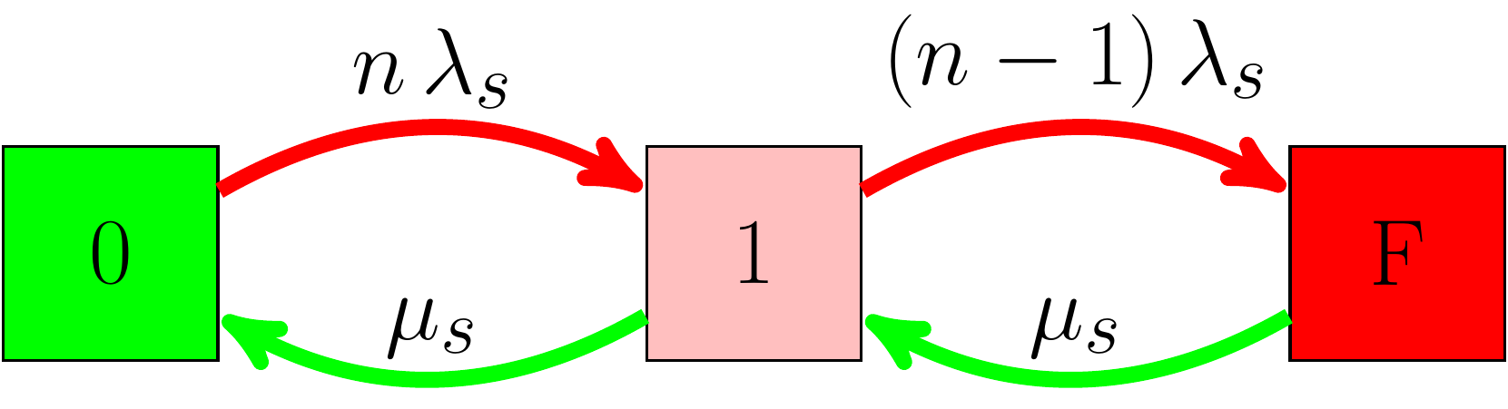
Markov Chain with one redundancy.
- With one redundancy, the data will be unavailable if \(2^+\) systems are down.
- Such a system can be modeled with the Markov chain shown on the left.
-
The availability can be computed as
\[\begin{equation} A_1=1-\left[n\frac{\lambda_s}{\mu_s}\right]\left[(n-1)\frac{\lambda_s}{\mu_s}\right](\#eq:a1pre) \end{equation}\]
The state equation in the \(s\)-domain is: \[\begin{equation} \begin{bmatrix} P_{n}(s) \\ P_{n-1}(s)\\ P_{n-2}(s) \end{bmatrix}=\mathcal{S}_1^{-1} \begin{bmatrix} 1 \\ 0\\ 0 \end{bmatrix}, (\#eq:avfull) \end{equation}\] where we defined \(\mathcal{S}_1\) as \[\begin{equation} \mathcal{S}_1=\begin{bmatrix} s +n \lambda_s & -\mu_s & 0 \\ -n\lambda_s & s +(n-1)\lambda_s +\mu_s &\color{red}{-\mu_s}\\ 0 &-(n-1)\lambda_s & s+\color{red}{\mu_s} \end{bmatrix}. (\#eq:smatrixav2) \end{equation}\] The terms in red show the additional terms compared to reliability analysis. Inverting the matrix and grabbing \(P_{n-2}\), we get \[\begin{equation} \frac{s^{-1}\lambda_s^2n (n-1)}{\mu_s^2-\lambda_s^2 n + \lambda_s \mu_s n + \lambda_s^2 n^2 - [\lambda_s + 2 \mu_s + 2 \lambda_s n ]s + s^2}. (\#eq:av1) \end{equation}\] We can expand \(P_{n-2}(s)\) in partial fractions, and there will be \(3\) poles: \(s_1=0\), \(s_{2,3}=\mu_s \pm \frac{1}{2} \lambda_s(n-1) + \sqrt{\lambda_s^2 +4 \mu_s\lambda_s (n-1)}\). Note that the poles \(s_{2,3}\) will result in exponential functions \(e^{-\mu_s t}\) decaying very fast, so we can just ignore them. So all we need is the coefficient of the pole at \(s=0\), let’s call it \(c_0\), which is easy to calculate: \[\begin{eqnarray} C_0&=&\lim_{s\xrightarrow{} 0} s P_{n-2}(s)=\frac{\lambda_s^2n (n-1)}{\mu_s^2 + \lambda_s \mu_s n + \lambda_s^2 n(n-1) }\nonumber\\ &\simeq& n(n-1)\frac{\lambda_s^2}{\mu_s^2}. (\#eq:coef) \end{eqnarray}\] Therefore the availability for a system with one redundancy is \[\begin{eqnarray} A_1&=&1-p_{n-2}(t)\simeq 1-C_0=1-n(n-1)\frac{\lambda_s^2}{\mu_s^2}\nonumber\\ &=&1-\left[n\frac{\lambda_s}{\mu_s}\right]\left[(n-1)\frac{\lambda_s}{\mu_s}\right],(\#eq:a1) \end{eqnarray}\] where we factored out the subtracted term to highlight a pattern. As an extra redundancy is added, the subtracted term is suppressed by a factor of \(\frac{\lambda_s}{\mu_s}\).Availability with \(c\) redundancies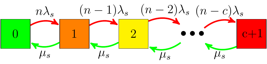
Markov Chain with \(c\) redundancies.
Recognizing the patterns in Eqs. @ref(eq:a0pre) and @ref(eq:a1pre) we can generalize the formula to a system with \(c\) redundancies: \[\begin{equation} A_c\simeq 1-\frac{n !}{(n-c-1)!}\left[\frac{\lambda_s}{\mu_s}\right]^{c+1} (\#eq:avgc) \end{equation}\]
Durability with Mach2
A mock up MACH2 drive with two actuators.
- The reliability of RAID critically depends on the speed of the recovery.
- MACH2 doubles the data transfer \(\implies\) 2x/4x reliability improvement for RAID5/6.
An interactive plot showing the gains with MACH2. … [+]
Durability with ReMAN
-
Consider with the simplest case[14]: one redundancy. Given a head/drive failure, there are two paths to losing data:
- A second failure while recovering from a head failure: less likely due to faster recovery.
- A second failure while recovering from a drive failure: more likely due to longer recovery.

Markov chain split into two parallel paths: recovery from subcomponent failures and recovery from device failures.
-
The plot on the left shows two parallel Markov chains:
- Left-most shows data recovery for a ReMan’able failure.
- Right-most shows the standard recovery when a drive fails.
-
\(r_m\) term represents the maximally ReMan’ed drive population.
- ReMan’able failures on maximal drives trigger replacement.
- This is represented by the dashed red curves.
- The transition rates are time dependent, and involve \(r_m\) functions.
-
\(\mathcal{R}^{(1)}_1(t)=exp\Big(-\frac{\mathcal{C}}{2 \Gamma}\left[t+\frac{1-e^{-2 \lambda_\mathrm{R} t}}{2 \lambda_\mathrm{R}}\right]-\frac{\mathcal{C}}{2\mu}\left[ (1+2 \kappa)t-\frac{1-e^{-2 \lambda_\mathrm{R} t}}{2\lambda_\mathrm{R}}\right]\Big)\) where \(\mathcal{C}\equiv n^2\lambda^2_{\mathrm{R}}(1+\kappa)\), and \(\kappa\equiv\frac{\lambda_\mathrm{NR}}{\lambda_\mathrm{R}}\)
- \(n:\) number of drives in the EC scheme, \(N:\) number of heads per drive,
- \(\Gamma:\) ReMan Repair rate, \(\mu:\) drive repair rate, \(\lambda_R\): ReMan’able failure rate, \(\lambda_{NR}\): non-ReMan’able failure rate.
- This is the expression when we allow for 1 ReMan/drive. Similar formulas are calculated for \(R_{max}=2,3\).
- We have an analytical model of Erasure Coded systems that support ReMan.
- The closed mathematical form can be computed instantly enabling a real-time web application.
- Multi-Layer EC
-
Improving data durability with